Mathematica Assignment:
The natural logarithm and exponential
Mathematica Assignment:
The natural logarithm and exponential
The natural logarithm and exponential
Danny Bell
MATH 162 [section]
08/07/2023
MATH 162 [section]
08/07/2023
Instructions: Your notebook should be both executable and human readable. Include all appropriate input cells (for your Wolfram language code), output cells (for your results), and text cells (for your analysis of results) in the proper order. In the final product, all input cells should be Wolfram language, not natural language cells. You will be penalized for missing, extraneous, or broken code. Additionally, you will penalized for missing analysis and poor grammar. Unless explicitly directed to perform a calculation by hand, all tasks should be performed by Mathematica using appropriate Wolfram language code. Intermediate results should be appropriately stored and accessed. In particular, try to avoid the very bad habit of copying output and pasting it as input into another cell. The ReplaceAll routine or /. operator is useful for accessing expressions that are returned as “rules” (e.g., the results of a call to the Solve routine). Whenever appropriate be sure to include legends and labels on axes for all plots.
1
. Consider the function .
f(x)=ln(x+1)
1
.1
.Compute the linearization of at .
f
x=0
In[]:=
x0=0f[x_]=Log[x+1];y0=f[x0]Lf[x]=y0+f'[x0]*(x-x0);Print[StringForm["The linearization of f at x0= `` gives ``.",x0,y==Lf[x]]]
The linearization of f at x0= 0 gives yx.
The output we are given for the linearization at x = 0 is y = x.
1
.2
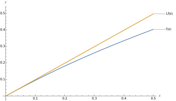
.Graph together with its linearization over the interval . Where does the approximation seem best? Where is it least good? Does the approximation overestimate or underestimate? Estimate the maximum absolute error involved in approximating by its linearization over this interval.
f
[0,1/2]
f
In[]:=
{a,b}={0,1/2};f[x_]=Log[x+1];Lf[x_]=y0+f'[x0]*(x-x0);Plot[{f[x],Lf[x]},{x,a,b},AxesLabel{x,y},PlotLabelsAutomatic,ImageSizeLarge]
Out[]=
The approximation seems best at x=0 which was the hope. The approximation seems to be the least good at x=0.5. We can see from the graph that the approximation overestimates the actual values of f(x). We can estimate the maximum absolute error on the interval (0 , 0.5) is 0.1.
2
. Consider the function .
f(x)=
x
e
2
.1
.Compute the linearization of at .
f
x=0
In[]:=
x0=0f1[x_]=E^x;y0=f1[x0]Lf1[x]=y0+f1'[x0]*(x-x0);Print[StringForm["The linearization of f at x0= `` gives ``.",x0,y==Lf1[x]]]
Out[]=
0
Out[]=
1
The linearization of f at x0= 0 gives y1+x.
2
.2
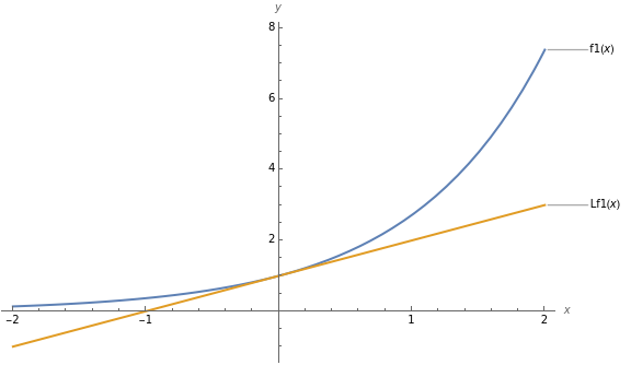
.Graph together with its linearization over the interval . Where does the approximation seem best? Where is it least good? Does the approximation overestimate or underestimate? Estimate the maximum absolute error involved in approximating by its linearization over this interval.
f
[-2,2]
f
In[]:=
{a,b}={-2,2};Plot[{f1[x],Lf1[x]},{x,a,b},AxesLabel{x,y},PlotLabelsAutomatic,ImageSizeLarge]
The approximation seems to be best at x = 0 which is what we were hoping would happen . We can see here from the graph that the approximation seems to be the least good at x=2. We can see that the approximation is an underestimate. The maximum absolute error involved in approximating x by its linearization over this interval is roughly 4.
The approximation seems to be best at x = 0 which is what we were hoping would happen . We can see here from the graph that the approximation seems to be the least good at x=2. We can see that the approximation is an underestimate. The maximum absolute error involved in approximating x by its linearization over this interval is roughly 4.

